A correlation matrix with fifteen rows gives you 105 unique pairwise cells and no way to hold them in your head at once. The question a risk committee actually asks is simpler than any individual cell. If the book runs fifteen exposures, how many genuinely different bets is that? The eigenvalue decomposition answers that in one number, and the number is usually smaller than the position count by a margin that is uncomfortable to write down.
I run this calculation before I run anything else on a matrix, because it tells me whether the rest of the analysis is worth doing. A book with an effective count near its position count has a real diversification story to tell. A book where the count collapses has one bet wearing several tickers, and every subsequent risk number is describing that one bet with more decimal places than it deserves.
Three models that turn out to be one and a half
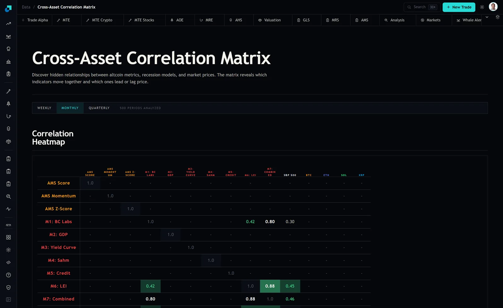
Take a worked example straight off the grid. At the time of writing the Cross-Asset Correlation Matrix was sitting on its MONTHLY window with 500 periods analyzed, and the recession-model block was the only region of the heatmap carrying readings. M1 (BC Labs) against M6 (LEI) read 0.42. M1 against M7 (Combined) read 0.80. M6 against M7 read 0.88. Everything else in those rows was a dash.
Treat those three models as three positions of equal size and equal volatility. The correlation matrix is the three-by-three block with ones down the diagonal and 0.42, 0.80 and 0.88 filling the rest. Its eigenvalues come out at 2.417, 0.583 and 0.0004. They sum to three, as they must for a correlation matrix, and the first one alone carries 80.6 percent of the total variance.
That third eigenvalue is the finding. A value of 0.0004 says the third dimension is essentially empty. Given M1 and M6, you can reconstruct M7 to within rounding. The panel labels M7 as Combined, and the decomposition behaves the way a composite built from the other models would behave. Anyone holding all three and describing it as three-model confirmation is describing the same signal twice and then averaging it.
The participation ratio, and what it will not tell you
The effective number of bets I use is the participation ratio of the eigenvalue spectrum. Square each eigenvalue, sum the squares, and divide the square of the total by that. For the block above the arithmetic is 9 divided by 6.182, or 1.46. Three positions, one and a half bets.
Two properties make this the version I put in a risk pack rather than the alternatives. It needs no threshold, so nobody argues about whether the cutoff should be 90 percent or 95 percent of variance explained. And it degrades smoothly, so a book that drifts from 4.1 to 3.6 over a quarter shows the drift rather than snapping between integer answers.
The entropy-based version of the same idea gives 1.64 on the same block. That gap is not an error in either method. The participation ratio penalises a dominant first factor harder than the entropy measure does, so it reads lower on concentrated spectra. Pick one, write the definition into the risk policy, and never quote the two interchangeably in the same document. I have watched a committee spend twenty minutes on a difference that was entirely a definition change.
The larger caveat is that this number is basis dependent. It counts independent directions in the space you handed it, so it answers the question you asked and not a question about the world. Feed it a matrix of five recession models and it will tell you about recession models. It cannot tell you that the whole block is one macro bet with no equity, credit or rates exposure in it at all.
Adding an asset class moves the count more than adding a model
Extend the block with the S&P 500 row, which was the fourth populated row at capture. It read 0.30 against M1, 0.45 against M6 and 0.46 against M7. Four positions now. The eigenvalues become 2.708, 0.753, 0.539 and 0.0004, the first factor drops from 80.6 percent to 67.7 percent, and the effective count rises from 1.46 to 1.95.
One additional position bought roughly half a bet. A fourth recession model correlated 0.85 with the existing three would have bought almost nothing. This is the practical use of the statistic in an allocation meeting. It converts the vague argument about whether a candidate adds diversification into an arithmetic before and after, and the answer is a number you can put next to the fee.
The same test applies to a manager search. Run the count on the existing roster, run it again with the candidate included, and the difference is the diversification the allocation is actually buying. If the count moves by 0.05, the case has to be made on expected return alone, because there is no diversification case left to make.
Six populated cells out of 105
The decomposition has a hard precondition that pairwise reading does not. You cannot decompose a matrix with holes in it. Of the 105 unique pairs available across the fifteen rows on the panel, six carried a coefficient at capture. The AMS block, the four crypto rows and most of the recession models showed dashes against each other.
A dash is missing data, not a zero. The difference matters enormously here, because filling holes with zeros does not produce a conservative estimate. It produces an estimate that overstates diversification, since every fabricated zero is an assertion of independence you have no evidence for. That failure runs in exactly the direction that flatters the book, which is the direction to be most suspicious of.
So the working discipline is to restrict the decomposition to the complete sub-block, and to report the coverage alongside the count. An effective count of 1.95 computed across four rows out of fifteen is an honest sentence. The same number presented as a portfolio-level diversification statistic is not, and the difference will surface in a review at the worst possible moment.
Putting the count into the monthly risk pack
The format I use has four fields and fits on one line. Universe and coverage, so the reader knows what was in the calculation and what was excluded for missing cells. Window, because the same book gives different counts on the weekly, monthly and quarterly toggles and the pack has to name which one it used. The count itself. And the change since the prior report.
The change field is where the value sits. A count that falls from 5.2 to 3.4 without any trade having been done is the matrix telling you the market re-correlated underneath a book you did not touch. That is a genuine risk event with no transaction attached to it, which means nothing in the trade blotter will ever surface it. It is also the single most useful thing to have written down and dated when a drawdown arrives and somebody asks whether the concentration was visible in advance.
Set a review trigger rather than a hard limit. A limit on an estimated statistic invites the estimation to be nudged, and the count is sensitive to window choice in a way that makes nudging easy. A trigger that says a fall of more than one full bet in a month goes on the agenda is harder to game and produces a better conversation, because the answer is sometimes that the re-correlation is transient and the right action is none.