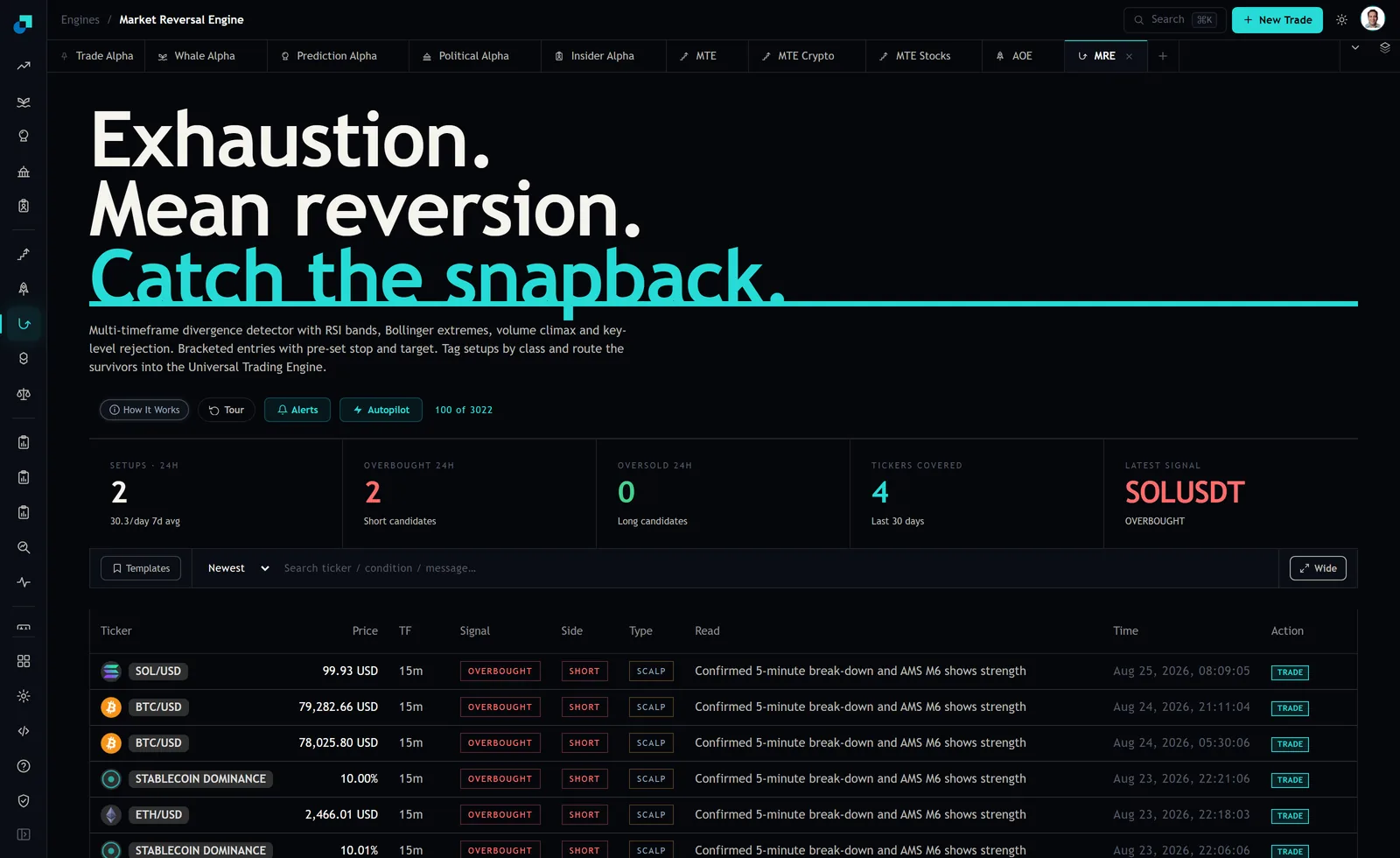
The visible MRE feed at capture was uniform in a way that matters for this question. Every row read 15m in the TF column and SCALP in the Type column, on BTC/USD quoted at 79,282.66 and ETH/USD at 2,466.01. That combination, a fifteen minute reversal held for a scalp window, is the hardest case in the module for capacity, and it is the one where the standard capacity estimate is most badly wrong.
Why average daily volume is the wrong denominator
The usual rule of thumb, take some small percentage of average daily volume, encodes an assumption that you get the whole day to work the order. A scalp reversal does not get the whole day. It gets the window between the signal print and the bracket resolving, which on a 15m setup is measured in bars. Liquidity you cannot reach inside that window is liquidity you do not have, and quoting it in a capacity memo is quoting someone else's trading day as though it were yours.
There is a second and less obvious problem. The engine looks for volume climax and key-level rejection among its triggers, which means the signal bar is selected for being an unusual bar. The book at that moment is not the book at a random moment. It is a book that has just absorbed a burst of one-directional flow, and it is thinner on the side you want and deeper on the side you are leaving. Average depth across all bars overstates the depth available at exactly the bars the strategy trades.
The combination of the two is why ADV-based capacity numbers for reversal strategies come out flattering, sometimes by an order of magnitude. The correction is not a fudge factor. It is measuring the right thing.
Measuring depth at the signal bar
The quantity you want is D(c), the notional executable within c basis points of the touch, aggregated across the venues you can actually route to, sampled at the signal timestamps rather than on a schedule. Three details make the difference between a number you can defend and one you cannot.
Sample at signal times, not at intervals. You have a list of timestamps from the archive, so use them. A depth series sampled every minute and averaged answers a question nobody asked.
Aggregate only reachable venues. Depth on an exchange you do not have an account, a credit line or a custody path to is not your depth. For crypto in particular this cuts hard, because the visible consolidated book across all venues can be several times the book available to any one participant with real operational constraints.
Sample both sides separately. The entry side and the exit side of a reversal trade are different sides of the book, and the whole point of an exhaustion signal is that they are asymmetric at that moment. A single mid-book depth figure hides the asymmetry that determines your cost.
Report the distribution, not the mean. The tenth percentile of D(c) across signal bars is a more useful capacity input than the average, because capacity constraints bind on the bad draws and the bad draws are correlated with the days you are carrying the most risk.
The stop exit sets the number, not the entry
This is the part most capacity work gets backwards. Entry into a reversal is a passive, patient action: the setup ships with a bracket, you have a defined level, and you can work the entry with limit orders inside the confirmation window.
The stop is not patient. A bracket stop fires into the direction that has just gone against you, at the moment that direction is running, which is precisely when the book on your exit side is thinnest. Sizing capacity off entry depth and then discovering exit capacity during your first bad week is a well-worn path.
The defensible construction measures D(c) on the exit side, conditional on the stop being triggered, and uses that as the binding constraint. Suppose your measured tenth-percentile exit depth within ten basis points on BTC at signal bars is three million dollars, and on ETH it is closer to nine hundred thousand. Those are placeholders and yours will differ, but carry them through. If your risk framework caps a single scalp position at three percent of gross, the BTC leg supports a gross book of about one hundred million and the ETH leg about thirty million. The strategy's capacity is the smaller one if you insist on running both legs at equal weight, and the difference is a reason to weight them unequally rather than a reason to average them.
Apply a stress multiplier on top. If exit depth under stress is a third of its median, the constraint tightens by the same factor, and a book sized on median depth will be discovering that during a liquidation cascade.
Clustered signals do not add capacity
The dashboard averaged 30.1 setups a day at capture. It is tempting to treat frequency as a capacity multiplier: more signals, more chances to deploy, more assets under management supported. That inference fails when signals cluster, and in this feed they visibly do.
The top two rows are both BTC/USD, both 15m, both OVERBOUGHT and SHORT, both SCALP, carrying identical Read text, timestamped about sixteen hours apart. Five visible rows share one Read string across three instruments. Signals that arrive in a cluster on correlated instruments do not give you independent positions to size independently. They give you one exposure, financed several times, with a single common exit.
The practical adjustment is to define capacity on the aggregate position the cluster implies rather than on the per-signal clip. Group signals into episodes by instrument, side and time window, size the episode, and treat additional signals inside the episode as information about conviction rather than as new deployments. A capacity number computed per row and multiplied by rows per day will overstate the real figure by whatever the clustering factor turns out to be, which is a number you can measure directly from the archive.
The crowding haircut you cannot measure
MRE delivers signals through a live dashboard, email alerts, and Discord and Telegram channels, and the module states that new signals surface within seconds of computation. Every subscriber receives the same instrument, the same side and the same bracket levels at effectively the same moment.
That has a specific consequence for capacity work: the depth you measured historically at signal bars includes whatever crowding already existed at that subscriber base, and it will not include the crowding your own participation adds, nor any future growth in the subscriber list. You cannot observe the counterfactual book, so you cannot measure this directly. What you can do is treat every capacity figure derived this way as an upper bound, state that explicitly in the memo, and build a monitor that would detect the constraint tightening.
That monitor is realised slippage at the signal bar, tracked over time against your own clip size. If slippage per unit of clip trends upward while your size is flat, either the venue liquidity has deteriorated or the signal has become more crowded, and the two are not distinguishable from your seat. Both call for the same response, which is to cut size on the affected leg. Setting that trigger before you scale is the difference between a capacity estimate that is a document and one that is a control.