The mechanism behind this idea is sound, which is exactly why it needs a strict test rather than an enthusiastic one. Correlations across risk assets rise when common factors dominate idiosyncratic ones, and common factors dominate when leverage is being unwound, liquidity is being withdrawn, or a single macro variable is driving everything. Those are the conditions a de-risking rule exists to catch. If average pairwise correlation moves before price does, it is a leading indicator worth building.
The word before is doing all the work in that sentence, and it is the part that usually fails. This is a specification for testing the claim properly, and I want to be direct about the boundary of the article at the start. I am not going to report a lead time, a false positive rate or a surviving threshold, because I do not have a study in front of me that I can stand behind and inventing those numbers would be worse than useless. What follows is the design that would produce them, and the arithmetic that will tell you whether the answer can be good enough to act on before you spend a month finding out.
The input, and where the panel leaves off
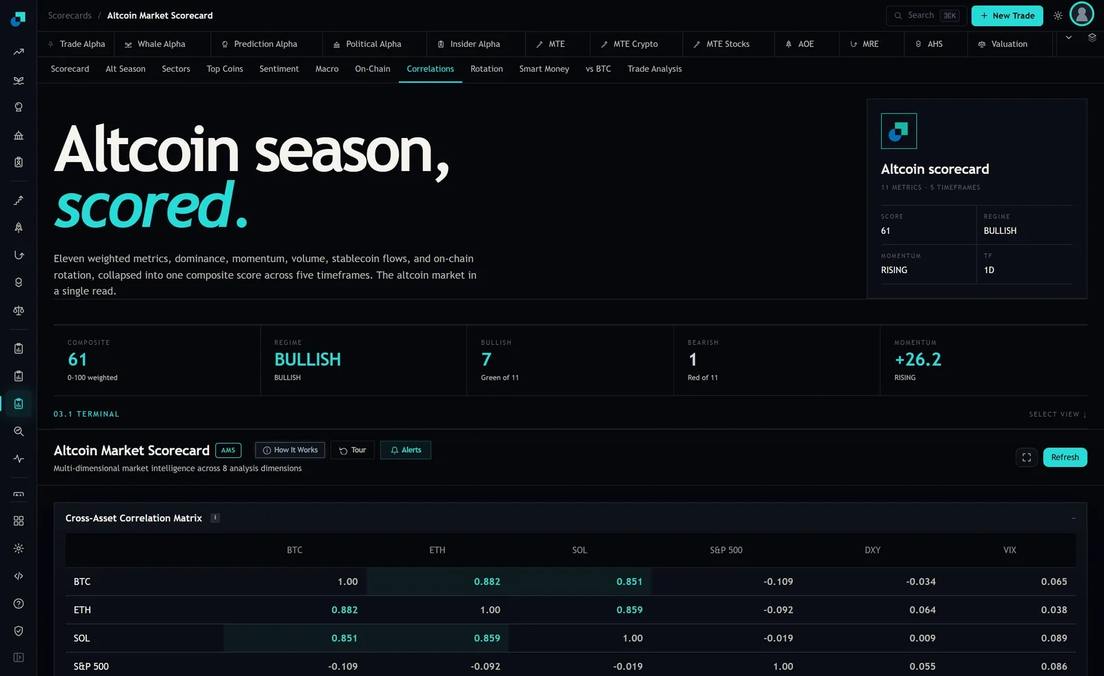
The Correlations tab of the altcoin scorecard prints a Cross-Asset Correlation Matrix. On this capture the crypto cells read BTC to ETH 0.882, BTC to SOL 0.851 and ETH to SOL 0.859, averaging 0.864. The module describes this dimension as cross-asset correlation matrices and regime detection.
What the panel gives you is a current reading over a small, fixed set of assets. What it does not give you, and what I cannot confirm exists anywhere on it, is a time series of average pairwise correlation, an adjustable estimation window, or any backtest of a threshold rule. A trigger test needs years of the series, not one value, so the panel's role here is a live cross-check on your own pipeline rather than the data source for the study.
Note the level while you are looking at it. An average of 0.864 across three majors is high in absolute terms. Any threshold you propose has to sit somewhere in the upper part of a range the series already occupies most of the time, which compresses the space available for a signal and is the first hint that this will be harder than it sounds.
Specifying the trigger before you look at anything
Write the full specification down and date it before running a single backtest. Every ambiguity you leave open is a degree of freedom you will unconsciously spend on making the result look good.
The specification needs six elements. The universe and its membership rule, fixed as of each date rather than selected from survivors. The return frequency. The estimation window length. The statistic, which is the equal-weighted mean of off-diagonal pairwise correlations, and whether it is a level or a change over some interval. The trigger condition, threshold or rate of change. And the action, which must be specific enough to price, meaning what fraction of the book comes off, over how long, and back on under what condition.
The action element gets skipped and it is the one that determines everything. A signal that is right about direction but triggers a round trip you cannot execute inside a week is not a trigger, it is an observation.
The three numbers the test has to produce
Lead time. Define the event first, from price and independently of the signal, using a rule like a drawdown of a stated depth in the benchmark within a stated horizon. Then measure the gap from first trigger to event onset. Report the whole distribution rather than a mean, because a trigger with a median lead of eight days and a wide left tail that includes negative values is coincident, not leading, and the mean will conceal that.
Expect this one to be uncomfortable. Correlation rises partly because deleveraging is already happening, which makes the signal endogenous to the event you want to front-run. Structural short lead time is the most likely honest finding here, and finding it is worth more than a rule that fails later.
False positive rate. The count of triggers not followed by an event within the horizon, divided by all triggers. Report the raw count too. A rate of twenty percent means something very different across five triggers than across a hundred.
The threshold. And with it, the full list of thresholds tested, because that list is the honest measure of how much searching produced the winner.
Base rate arithmetic decides this before the backtest does
Run this arithmetic first. It takes five minutes and it will frequently tell you not to bother.
Suppose events worth de-risking for occur in eight percent of months. Suppose your trigger catches seventy percent of them and fires on twenty percent of the quiet months. Then the probability that a trigger is followed by an event is 0.08 times 0.7, divided by that quantity plus 0.92 times 0.2. That is 0.056 over 0.240, or about 23 percent.
Those are illustrative inputs, not measurements, and the point of the exercise is the shape rather than the value. A trigger with a respectable hit rate and a modest false positive rate is still wrong roughly three times in four when it fires, because the event is rare. That is not a flaw in the indicator. It is what conditioning on a rare outcome does, and it holds for every risk-off signal anyone has ever built.
So the decision is not whether the trigger is usually right. It is whether the cost of being wrong three times in four is smaller than the loss avoided the fourth time. Price that directly. Cost per false positive is round trip execution plus the expected return given up while out of the market, in basis points of the sleeve. Multiply by expected false positive frequency per year. Compare against avoided drawdown times true positive frequency. If that comparison is close, the strategy is not viable, because your parameter estimates are not precise enough to distinguish close from negative.
What counts as surviving out of sample
The threshold scan is where this fails quietly. Nine thresholds crossed with three window lengths and two universe definitions is fifty four configurations, and the best of fifty four looks excellent in sample by construction. A single out-of-sample period does not fix that, because the choice of which configuration to carry forward was already made on the full history.
Three defences, in order of strength. Walk forward, selecting parameters only on data prior to each evaluation window, which is the minimum acceptable standard. A parameter stability check, since a threshold that works at 0.75 and fails at 0.70 and 0.80 is a fitted artefact regardless of its statistics, while a broad plateau of comparable performance is the shape of something real. And a shuffle test on the trigger dates, preserving the count and clustering while destroying the timing, to establish what your performance metric looks like with no information at all.
Then document the negative result if that is what you get, and keep it. A desk that has actually tested this and written down what it found is in a stronger position than one that keeps rediscovering the idea every eighteen months and rebuilding the same backtest, and the second desk is far more common than the first.