Most crypto event studies are equity event studies with the exchange calendar quietly removed. The estimation window is still a few hundred observations, the event window is still a day or two either side, the abnormal return is still a residual against a market proxy, and the whole apparatus is now running on a market that never closes and whose benchmark is one of the assets being studied.
The convention was not arbitrary. Each piece of it was buying something specific, and if you are going to keep the method you have to replace what the calendar was providing rather than assume you never needed it.
What the daily-close convention was actually buying
Four things, and it is worth naming them because each one has to be re-sourced.
Synchronisation. Every security in an equity sample is observed at the same instant, because the close is the same instant for all of them. Returns are therefore comparable across names without any alignment work, and cross-sectional averages mean something.
A natural unit and a natural gap. The trading day gives non-overlapping intervals of roughly equal information content, and the overnight gap gives a clean place for information to arrive and be impounded at the next open. Studies that anchor on a close are implicitly using that gap.
An accepted benchmark. There is a market portfolio that everyone in the field uses, it is measured on the same clock, and disagreements about it are about weighting rather than about existence.
A settled length convention. The estimation window of a few hundred trading days ending well before the event, and the short symmetric event window, are conventions rather than results, but they are shared conventions, which is most of their value. Everyone knows what a two-day window means without asking.
A continuous market supplies none of these for free.
Lookback columns are not event windows
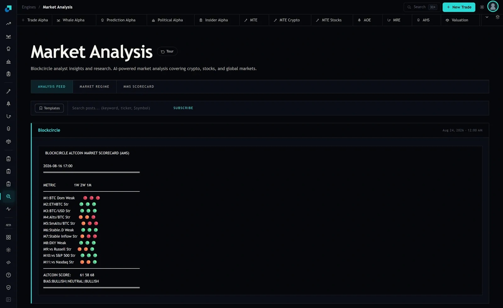
The capture above is a useful contrast case rather than a target. Its horizons are calendar spans, which is already more honest for a continuous market than trading-day counts would be, and the single stamp beneath the title is the anchor for all three. But it is describing state, and turning a state description into an event study requires two things it does not have: an event to anchor on, and a model of expected return over the same interval.
The missing timezone on that stamp is the small detail worth stealing as a rule. In a market with no close, a timestamp without a zone is not a timestamp. Every window definition your house writes should carry an explicit zone, and the sensible choice is UTC everywhere, converted only at the point of display, because the alternative is a research library where half the studies silently shift by an hour twice a year.
Estimation and event windows measured in hours
Rebuild the convention in units the market actually has. Hourly bars are usually the right granularity for anything above the microstructure layer, and they give you an integer count for every span.
Set the estimation window as a fixed number of hourly observations ending a stated gap before the event, with the gap doing the job the equity convention's thirty-day buffer did: keeping anticipation and leakage out of the sample used to define normal. In a market where positioning moves in front of scheduled events, a longer gap is defensible and the length should be stated rather than defaulted.
Set the event window asymmetrically. The equity habit of a symmetric window around the day exists because the day is the unit. On a continuous clock there is no reason for symmetry, and there is a strong reason against it: the pre-event side is there to detect leakage and the post-event side is there to measure impounding, and those have different natural lengths. A short pre-window and a longer post-window is the usual shape.
Then fix the horizons in advance and publish them. The failure mode this prevents is the one that destroys credibility fastest, which is a study whose window length was chosen after the abnormal returns were seen. In a market with no calendar there is nothing stopping a researcher from trying eleven window lengths, so the discipline has to come from the process. Pre-register the set of windows your house reports, report all of them every time, and treat any additional window as an exploratory result that is labelled as such.
What plays the role of the market portfolio
The benchmark question is harder in crypto than in equities and it does not have a clean answer, so the requirement is that the choice is deliberate and disclosed rather than inherited from whatever the library defaults to.
Three workable constructions, each with a known weakness. A single dominant asset as the market factor is simple and observable, but it is itself frequently the subject of the events being studied, and using it as a benchmark for an event that moves it will null out exactly the effect you are measuring. A capitalisation-weighted basket is closer to the equity analogue, but its weights are dominated by the same asset and its composition changes underneath you. A sector or peer-matched basket controls best for the shared component and is the most vulnerable to selection, because the peer set is chosen by the researcher.
Whichever you pick, estimate the relationship on a rolling basis rather than a fixed one. Beta against a dominant asset is not stable across regimes, and an estimation window from a quiet period applied to an event in a volatile one produces residuals that are mostly a beta error. Rolling estimation with the window length disclosed is the minimum, and reporting the estimated beta alongside the abnormal return lets a reviewer see when the model was straining.
Denomination is a separate decision that gets skipped. Returns measured against a stablecoin and returns measured against a fiat reference are not the same series during stress, and a study that mixes them across its sample has an unstated factor in it.
The hour of the week is structure, not noise
Continuous does not mean homogeneous. Liquidity, spreads and depth vary systematically by hour of the day and day of the week, driven by which regions are awake and which traditional venues are open. Weekend hours behave differently from midweek hours in ways that are persistent enough to be modelled rather than averaged away.
This has a direct consequence for windows. An event landing at a thin hour will show a larger price response for the same information content, because the same order flow moves a shallower book. A study that pools events across all hours and reports one average abnormal return is reporting a mixture of information effect and liquidity effect, weighted by the accidental hour distribution of its sample.
The corrections are ordinary. Include hour-of-week effects in the expected return model, or draw the estimation sample from matched hours rather than from the immediately preceding block, and report the hour distribution of your event sample so a reader can see whether it is concentrated. Where the sample allows it, split results into liquid-hour and thin-hour subsamples. A result that only exists in the thin-hour subsample is usually a capacity story rather than an alpha story, and better to find that in research than in production.
Overlapping events and the standard errors nobody adjusts
The last piece is where crypto event studies most often overstate significance. Events in this market cluster hard: a macro print, a large liquidation cascade and a protocol announcement can land inside the same six hours, and the affected assets are all loaded on the same dominant factor.
When event windows overlap in calendar time, the abnormal returns are cross-correlated and the usual standard errors are too small. The result is a t-statistic that looks decisive on a sample that contains, in effect, far fewer independent observations than the row count suggests. In a market with high shared factor loading this is not a marginal correction.
The practical responses are to cluster by calendar period, to aggregate into a calendar-time portfolio and test on the portfolio series rather than on individual events, or to bootstrap using blocks that preserve the clustering. Whichever you use, report the number of distinct calendar periods alongside the number of events, because that pair of numbers tells a reviewer in one glance how much independent evidence is actually in the study.