Every deployment underperforms its backtest. That is not a finding, it is the base rate, and reporting it as a headline number tells a committee nothing they can act on. The useful version splits the shortfall into buckets that have different owners. Commission is a broker negotiation. Spread is a venue and order type decision. Delay is an infrastructure problem. Alpha decay is a research problem, and it is the only one of the four that means the strategy itself is worth less than you thought.
The Momentum Trading Engine's trade log carries most of what the decomposition needs, and knowing exactly which fields it does not carry is as important as knowing which it does.
First remove the rows that were never traded
Before any arithmetic, filter the log. At capture the trades tab showed 357 trades and carried an explicit banner stating that 44 of the rows below had been reconstructed by replaying the strategy over historical candles, that no order was placed and no fill occurred for those rows, and that they show what the strategy would have done rather than what it did.
Roughly one row in eight is a simulation. Leave those in and you have put backtest rows on the live side of a live versus backtest comparison, which drives your measured gap toward zero and produces a reassuring report that means nothing. This is the single most consequential step in the whole exercise and it takes one filter.
The Source column is the field to filter on, and it is worth understanding what its values mean before you trust them. At capture an active Ford position carried a source of MTEAdopted, which describes how the position entered the log rather than how it was filled. Establish with the vendor which source values correspond to a real order and which do not, and write that mapping into the reconciliation script rather than into somebody's memory.
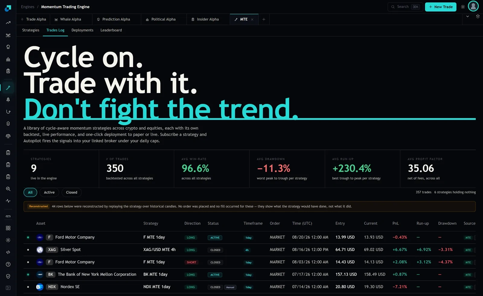
What the log carries, and the two fields it does not
The columns run Asset, Strategy, Direction, Status, Timeframe, Order, Time in UTC, Entry, Current, PnL, Run-up, Drawdown, Source and Duration. That is a rich log by vendor standards. It gives you the instrument, the side, the order type, a timestamp, an entry price and a realised or running return.
Two things are missing and both matter. There is no commission field, so bucket one has to come from your broker's execution file. And there is only one price on the entry side, which means the log does not separate the price the signal fired at from the price you were filled at. Without a decision price, the delay bucket cannot be read off the table and has to be reconstructed.
Check what the PnL column is measuring before you use it as the live number. On the Ford row at capture, entry was 13.99 and current was 13.93, and the displayed PnL was minus 0.43 percent. Work it and the difference over the entry price is minus 0.429 percent, which reconciles exactly. The PnL column is a clean price return computed off the two price fields, gross of every cost. That is the right convention for a signal log and the wrong number to report as live performance, because your realised result is that figure minus all four buckets.
Commission and spread, the two that come from outside
Commission is the simplest. Pull per-trade commission from the broker file, join on instrument and timestamp, and express it in basis points of notional. Do it per instrument, because a strategy library spanning crypto spot and futures, US equities, forex and commodities pays on four different fee schedules, and a blended average will hide the one that is destroying a sleeve.
Spread is a modelling choice rather than an observation. The Order column at capture read MARKET, which means you crossed. The cost of crossing is half the quoted spread at the moment of the fill plus whatever the book gave up beyond the touch. If you capture quote data at fill time, use it directly. If you do not, use the median quoted spread for that instrument in that time bucket and mark the bucket as estimated in the report, because an estimated component presented as measured is how these reports lose credibility.
The reason to keep these two separate rather than lumping them as transaction costs is that they have different fixes. Commission responds to a rate negotiation or a venue change. Spread responds to using limit orders, which changes the strategy's fill rate and therefore its signal, and that tradeoff belongs to research rather than to the trading desk.
Delay, and the midnight timestamp problem
This is where the log's structure does real work. The Ford position was on a one day timeframe with a signal timestamped at midnight UTC on the twentieth of August, with a market order, on a US listed equity.
A US equity cannot be filled at midnight UTC. The regular session opens more than thirteen hours later. So the interval between the timestamp the backtest treats as the decision point and the first moment a market order could actually execute spans an entire overnight session, including whatever gapped in it. That is the delay bucket, and on a daily bar strategy it is not a latency question measured in milliseconds. It is an overnight gap measured in figures.
Measure it directly. For each live trade, take the instrument's price at the signal timestamp, take the Entry price actually recorded, and the difference in the direction of the trade is your delay cost for that row. Aggregate in basis points and split by instrument and by timeframe. Expect the daily-bar strategies to carry the largest delay cost and the intraday ones the smallest, which is the reverse of what most people assume.
One caution about the Duration column. The Ford row showed five days and zero hours, quantised to whole days. Durations that land on exact day boundaries are being measured in bars rather than in clock time between fills, so the column will not give you intraday timing and should not be used as a latency input.
Alpha decay has to be measured, not left over
The tempting shortcut is to compute the total gap, subtract the three measured buckets, and call the remainder alpha decay. Do not. A residual absorbs every measurement error in the other three, every mismarked row, and every trade you failed to match to a broker fill. It will always be non-zero and it will always look like decay.
Measure it on its own terms. Take the strategy's rules and evaluate the return from entering at increasing lags after the signal, one bar, two bars, five bars, holding the exit rule fixed. The slope of return against entry lag is the decay curve, and the value at your measured average delay is the alpha decay attributable to being late. If the strategy loses forty basis points of edge per bar of delay and you are consistently one bar late, that is your number and it was derived rather than inferred.
Then reconcile. The four buckets should sum to within a small tolerance of the observed gap between the log's gross PnL and your realised P and L. When they do not, the discrepancy is almost always unmatched rows rather than a genuine fifth effect, and the usual culprit is a reconstructed row that survived the first filter. Run the reconciliation monthly per strategy, and treat a widening delay bucket as an operations ticket while a widening decay bucket goes to research with a recommendation to cut size, because those are the two findings that look identical in a headline number and require completely different responses.