Most concentration policies limit single names and stop there. Five percent per position, twenty percent per sector, done. The gap that leaves is not subtle. Six positions at four percent each, all correlated at 0.7, sit entirely inside a five percent single-name limit while behaving like one bet at a size no committee would have approved if it had been written as one line.
Correlation clusters close that gap, but only if the translation from cluster to cap is arithmetic rather than judgement. What follows is the formula I use, why it produces the right behaviour at both ends, and how to write it so a risk committee can review and sign it rather than nod at it.
Why a per-name limit does not bind
The variance of an equally weighted group of k positions with average pairwise correlation r has a closed form, and the useful way to read it is as an effective count. The group behaves like k divided by one plus k minus one times r independent positions.
Put numbers through it. Six names at r of 0.7 behave like 1.33 independent positions. At r of 0.5, like 1.71. At r of 0.3, like 2.4. At r of zero, like six, which is the case the per-name limit was silently assuming. The single-name limit is not wrong. It is answering a question about one position while the risk is being taken by a group.
From cluster to cap in one line
The cap follows directly. Set the cluster limit at the per-name limit multiplied by the effective count of the cluster. With a five percent single-name limit, a six-name cluster at r of 0.7 caps at 6.7 percent of the book. At r of 0.5 it caps at 8.6 percent. At r of 0.3, twelve percent. At r of zero, thirty percent, which is exactly six times the per-name limit, meaning the formula reproduces the old policy when the correlation assumption behind the old policy happens to hold.
The other boundary is the one that makes this defensible. As correlation approaches one, the effective count approaches one and the cluster cap collapses to the single-name limit, which is precisely right. Six perfectly correlated positions are one position and should be limited as one.
The behaviour in between is where the policy earns its keep. Hold r at 0.5 and grow the cluster. Five names give an effective count of 1.67, six give 1.71, eight give 1.78, twelve give 1.85. The ceiling is one divided by r, which is 2. Adding names to a correlated cluster buys almost nothing after the sixth. That single observation kills more bad diversification arguments than any other number in this article, because the pitch for the seventh name in a crowded theme is always that it adds breadth.
Name the effective-count definition or the policy will drift
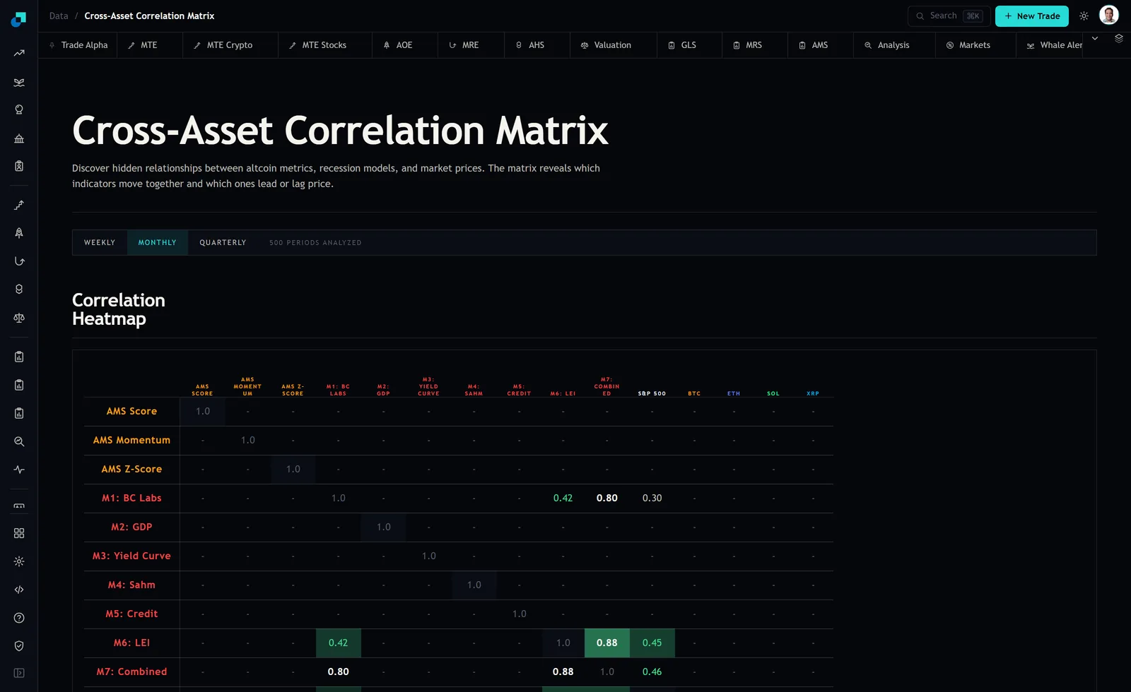
There is more than one statistic called an effective number of positions, and they do not agree. The variance-based count above gives 1.25 for a three-name cluster at r of 0.7. The eigenvalue participation ratio on the same matrix gives 1.52. On the actual three-model block that was populated on the panel at capture, with cells of 0.42, 0.80 and 0.88, the participation ratio gives 1.46.
A twenty percent spread between two defensible definitions is a twenty percent spread in every cap the policy produces. So the policy names one, defines it in an appendix with the formula written out, and forbids substituting the other in any document that references the limit. I use the variance-based count for limit setting because it comes straight out of the portfolio variance the limit is trying to control, and because it is the more conservative of the two on concentrated clusters.
The average correlation input needs the same treatment. Average the off-diagonal cells of the cluster in Fisher space, not raw, and state the window. On this panel that means naming the weekly, monthly or quarterly toggle, and it is not a formality. A cluster defined on one window can dissolve on another.
The four clauses that make the policy workable
The first clause defines cluster membership and the re-fitting cadence. Mine reads that clusters are re-fitted quarterly from the correlation matrix on the named window, using average linkage on correlation distance, cut at a height corresponding to an average within-bucket correlation of 0.50. Stating the cut as a correlation floor rather than a tree height is what makes the clause reviewable by a committee member who has never read a dendrogram.
The second clause fixes membership between re-fits. Without it, a position drifts out of a cluster on a Tuesday, the cap loosens, the desk adds, and the position drifts back on Friday into an automatic breach nobody caused. Membership is frozen at the re-fit date and changes only at the next one, or by an explicit intra-quarter decision that is minuted.
The third clause covers coverage. Clustering requires a complete sub-matrix, and matrices have holes. At capture, six of the 105 unique pairs across the fifteen rows on this grid carried a coefficient at all. Positions whose correlations cannot be estimated do not vanish from the risk report. They go into an unclustered bucket with its own cap, sized conservatively, because an unestimable correlation is an unknown, not a zero.
The fourth clause sets the tolerance. Estimated limits need a soft band, typically a passive breach zone of a couple of percentage points where the position is reported and reviewed but not force-reduced. Hard-stopping on an estimated statistic converts estimation noise into forced trading, and forced trading in a correlated cluster is the worst possible execution environment, since every name you are selling is moving with every other name you are selling.
Breaches with no trade behind them
The distinctive feature of a correlation-based limit is that it can breach while the book is untouched. Nobody traded, the market re-correlated, the cluster tightened, the effective count fell and the cap moved below current exposure. There is no entry in the blotter to point at.
Handle those explicitly, because the default assumption in any breach process is that somebody did something. The report should separate breaches into position-driven and correlation-driven, and the correlation-driven ones should carry the before and after effective count so the reader can see the size of the move. A cluster whose effective count fell from 2.4 to 1.5 in a quarter is telling you something about the regime that no position report will surface.
The remediation is different too. A position-driven breach is fixed by trimming. A correlation-driven breach might be fixed by trimming, or it might be a signal that the correlation estimate is unstable rather than that the risk has genuinely changed, in which case the right action is to check the same cluster on the other two window toggles before touching anything. That check takes a minute and it is the difference between a policy that improves the book and one that generates turnover during exactly the periods when liquidity is worst.
Log the decision either way. The dated record showing that the cluster tightened, that the committee saw it, and that the chosen action was to hold with a review trigger is worth more in the post mortem than the trim would have been.