Every mean-variance optimizer I have ever fed a raw sample correlation matrix has handed back a portfolio nobody would trade. Enormous longs, enormous offsetting shorts, and a stated risk number lower than anything the book has ever achieved. The instinct is to blame the optimizer. The optimizer is doing exactly what it was asked. The problem is upstream, in the matrix, and it is fixable with arithmetic that takes about a minute.
The fix is shrinkage. You pull the estimated coefficients partway toward a structured target, trading a small amount of bias for a large reduction in variance. The approach associated with Ledoit and Wolf formalises how far to pull. What follows is the mechanic worked on real cells, because the size of the effect is more persuasive than the theory.
What the optimizer does with an honest sample estimate
At the time of writing the Cross-Asset Correlation Matrix was on its MONTHLY window over 500 periods analyzed, and the recession-model block carried the only populated readings on the grid. M1 (BC Labs) against M6 (LEI) read 0.42, M1 against M7 (Combined) read 0.80, and M6 against M7 read 0.88.
Build the three-by-three from those three numbers, assume equal volatility so the correlation matrix is the covariance matrix up to a scalar, and solve for minimum-variance weights. The answer is 279 percent in M1, 352 percent in M6 and minus 531 percent in M7. That is the output of a correct calculation on a correct input, and it is untradeable.
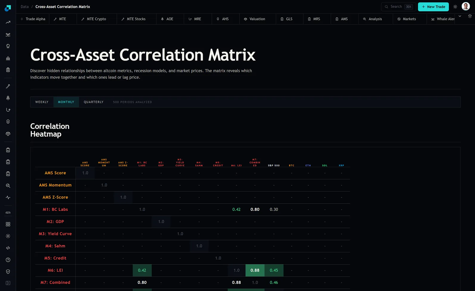
The diagnostic that explains the blow-up is the condition number, the ratio of the largest eigenvalue to the smallest. For this block it is 6,077. The smallest eigenvalue is 0.0004, which means one direction in the space carries almost no variance, and the inversion the optimizer performs divides by that near-zero. Any position the matrix considers a near-perfect hedge gets levered until the rounding error in the estimate becomes the dominant term in the answer.
The shrinkage dial and what each turn costs
The standard target for a correlation matrix is constant correlation. Take the average of the off-diagonal cells and replace every off-diagonal entry with it. Here the average of 0.42, 0.80 and 0.88 is 0.70, so the target is a matrix with 0.70 everywhere off the diagonal. The shrunk estimate is a weighted blend, intensity times the target plus one minus intensity times the sample.
Turning the dial produces this. At intensity 0.2 the minimum-variance weights come back as 80, 88 and minus 67 percent, and the condition number falls from 6,077 to 38.5. At 0.3 the weights are 63, 67 and minus 30 percent, condition number 25.8. At 0.4 they are 54, 55 and minus 9 percent, condition number 19.4. At 0.5 the short disappears entirely and the weights read 48, 48 and 4 percent, condition number 15.6.
Read that sequence carefully, because the first turn of the dial does most of the work. Going from zero to 0.2 removes 99 percent of the conditioning problem. Going from 0.2 to 0.5 removes a further fraction of what is left while progressively erasing the genuine information in the differences between 0.42, 0.80 and 0.88. By intensity 0.5 the estimator has decided that M7 is barely worth shorting, which is a strong opinion for a smoothing step to be expressing.
That is the cost side of the trade. Shrinkage is a bias you are deliberately introducing. If the sample matrix is telling the truth about a real structural relationship, shrinkage will pull you away from it, and no amount of stability will make that free.
Choosing the target before you choose the intensity
Most of the argument about shrinkage happens over the intensity parameter, which is the wrong argument. The target embeds a stronger assumption. A constant-correlation target says every pair is exchangeable, which is a defensible prior inside one asset class and an indefensible one across a matrix that mixes recession models with the S&P 500 and four crypto assets, as this grid does.
Across a mixed universe I prefer a block target. Compute an average correlation within each block and a separate average between blocks, then shrink toward that. It preserves the coarse structure you are confident about while smoothing the pairwise estimates you are not. The identity matrix as a target is available and I avoid it, because it shrinks toward the assumption of independence and therefore biases every diversification statistic in the flattering direction.
Whatever the target, calculate it inside the estimation window rather than importing a long-run average from somewhere else. A target computed on a different sample is a second estimate with its own error, silently added to the first.
Collinearity is not the same problem as sampling noise
The usual justification for shrinkage is short samples. With N series you are estimating N times N plus one, over two, coefficients, which for the fifteen rows on this panel is 120 parameters. The panel reports 500 periods analyzed, which is a comfortable ratio and not obviously a small-sample problem.
Yet the three-by-three block above blew up anyway, and it was estimated from the same 500 periods with only three parameters. That is worth sitting with. The instability there is not sampling noise. It is structural near-collinearity, and it would persist with an infinite sample, because M7 is labelled Combined and the block behaves the way a composite of its own components behaves.
The distinction changes what you should do. Sampling noise is a case for shrinkage. Structural collinearity is a case for dropping a series, because holding a composite alongside its components adds a redundant column and no information. Shrinkage will stabilise the weights either way, which is precisely the danger. It will produce a clean, plausible, well-conditioned answer to a specification that should never have been run.
So run the eigenvalue check first. If the smallest eigenvalue is near zero and you can point at the reason in the data dictionary, fix the specification. Reach for the estimator only when the instability has no structural explanation.
Documenting the estimator so the weights survive a review
Shrinkage is a discretionary choice inside a process that is supposed to be repeatable, so it has to be written down before it is used. Four things belong in the note. The target and why that target for this universe. How the intensity is set, whether by the analytic formula or by a fixed house value. The estimation window, which for this panel means naming the weekly, monthly or quarterly toggle. And the pre-shrinkage condition number, which is the evidence that the step was needed.
Keep the unshrunk weights next to the shrunk ones in the working papers. The gap between them is the honest measure of how much of the portfolio is coming from the estimator rather than from the data. When that gap is small, shrinkage was cheap insurance. When the unshrunk solution is minus 531 percent in a position and the shrunk one is minus 9 percent, the estimator is making the allocation, and everyone signing the recommendation should know that before the drawdown rather than during the post mortem.