The question that decides whether a macro liquidity overlay is investable at your size is not whether the signal has edge. It is how many times a year it asks you to trade, because that single number sets your turnover, your cost drag, your capacity ceiling and how much of the position you can move before you are the print. Get the trade count wrong by a factor of three and a strategy that clears a 2 bps hurdle becomes one that does not.
The input calendar caps the trade count
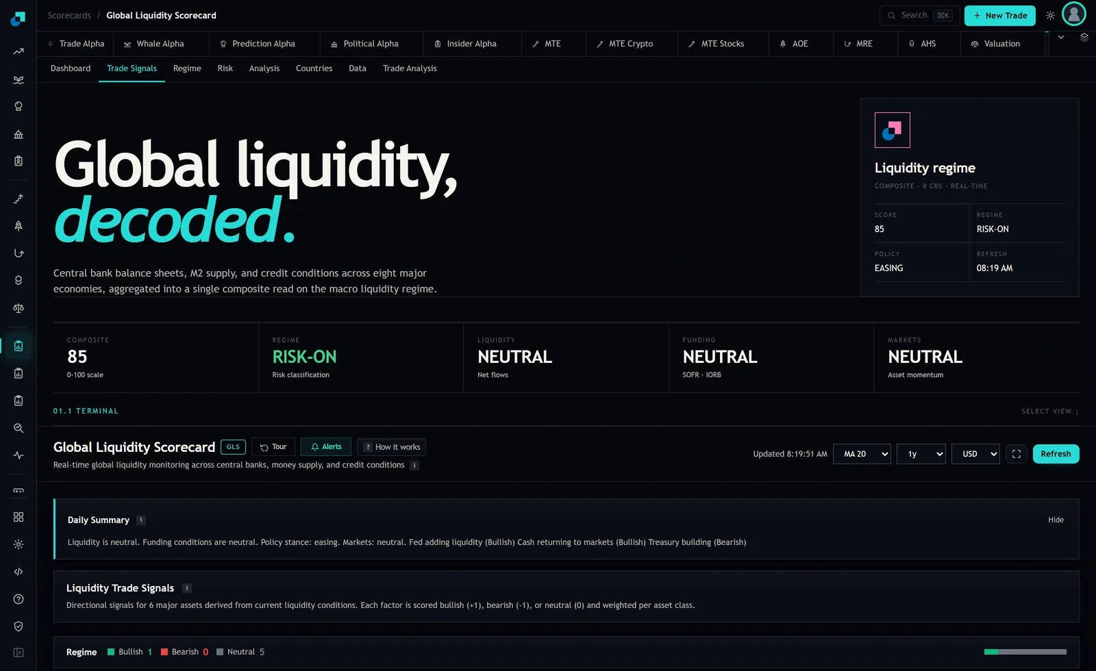
The Global Liquidity Scorecard aggregates eight central banks, the Fed, ECB, BoJ, PBoC, BoE, SNB, BoC and RBA, together with global M2, USD liquidity indicators and credit spreads, into a composite on a 0 to 100 scale. It currently prints 85 with a regime label of RISK-ON and a policy label of EASING.
Those inputs publish on weekly and monthly calendars. That imposes a ceiling on the information rate of the output that no amount of intraday recomputation can lift. The header carries the word REAL-TIME and a refresh stamp of 08:05 AM, and it is worth being clear with your investment committee about what that stamp means. It is the time the composite was last recalculated, not the time new information entered it. On the large majority of mornings the recomputation runs across an unchanged input set.
The practical consequence is that any decision rule built on this composite is structurally slow, and the useful engineering question is not how to make it faster but how many discrete exposure changes per year you should expect and budget for. That number is a policy choice you make when you set your bands, not a property of the data feed.
Turnover arithmetic at each candidate rebalance rate
Fix a convention so the numbers mean something. Define one exposure change as a 20 percentage point move in the overlay's target risk weight, so each change requires trading 20 percent of NAV in notional. Call the all-in execution cost per unit of notional c, expressed in basis points, covering spread, market impact and commission but not financing.
Annual notional traded is then 20 percent times the number of changes. Cost drag on NAV is that figure multiplied by c. The table is unromantic and it is the whole argument.
| Exposure changes per year | Notional traded, percent of NAV | Drag at c = 2 bps | Drag at c = 10 bps |
|---|---|---|---|
| 2 | 40 | 0.8 bps | 4 bps |
| 4 | 80 | 1.6 bps | 8 bps |
| 8 | 160 | 3.2 bps | 16 bps |
| 12 | 240 | 4.8 bps | 24 bps |
| 24 | 480 | 9.6 bps | 48 bps |
Read the table as a hurdle rather than a cost estimate. At four changes a year executed in liquid index futures at a couple of basis points, the overlay needs to add something over 2 bps a year to justify its existence, which is a low bar that a genuine regime signal should clear comfortably. At twenty-four changes a year executed in cash equities at ten, it needs close to 50 bps before it pays for itself, and now you are asking a monthly-frequency macro composite to produce half a percent of annual alpha net of everything. That is a materially harder claim to defend in a review.
The asymmetry is the point. The cost side of this scales linearly and predictably with trade count. The information side does not scale at all, because the underlying releases do not arrive more often just because you look more often. Every additional rebalance you allow yourself is a guaranteed cost against an unchanged information set.
Capacity is a property of the instrument, not the signal
A signal has no capacity. The implementation does. Once you have fixed the trade count, capacity falls out of what you trade and how long you are willing to take to trade it.
Work it from participation. If your policy is to take no more than 10 percent of average daily volume in the instrument you are using, and one exposure change is 20 percent of NAV, then a fund of size F needs 0.2F of notional executed. Spread across a three-day execution window at 10 percent participation, the strategy fits comfortably where 0.2F is small relative to three days of volume in the venue, and it starts to leak where it is not. Index futures on the major benchmarks absorb this at institutional size without much argument. A basket of single-name cash equities does not, and the same overlay run in crypto perpetuals faces a third set of constraints entirely, where depth is adequate on two or three names and thin on everything else.
This is why the low trade count is the capacity argument rather than a limitation. A slow overlay can take three days to move without the delay costing it anything meaningful, because a signal built from weekly and monthly data has no view on where prices are within a three-day window. A fast strategy cannot make the same trade, because the delay eats the edge. Slowness converts directly into execution flexibility, and execution flexibility converts directly into capacity.
What you cannot put in the memo
Now the honest limits, because these belong in the mandate documentation before the position does.
I cannot tell you how many exposure changes a year this composite has historically produced. The Trade Signals tab sits alongside Dashboard, Regime, Risk, Countries, Data and Trade Analysis in the module, and in the capture I am working from it shows the header, the composite and the two labels. It does not show me a signal history, a fired-alert log, a threshold, or a control for setting one. So I am not going to state a historical trade count or a hit rate, and you should treat any such figure that arrives without a point-in-time series behind it as unverified.
What that leaves you is a measurement task rather than a citation. Log the composite, the regime label and the policy label at a fixed time each week, in a file you control, and stamp each row with the date you observed it. After two or three quarters you can count how many times your own bands would have triggered, and that count is worth more than any vendor figure because it is point-in-time by construction and it reflects the bands you actually intend to run. Until then, size the overlay against the pessimistic row of the table rather than the optimistic one.
The related trap is revision. Monetary aggregates and balance sheet data get restated, so a composite recomputed today over restated inputs can show a cleaner path than anyone could have traded. Any backtest of this that does not use vintage data will overstate the trade count in the calm stretches and understate it around turns, which is precisely the wrong direction for a capacity estimate.
Crowding, and why slowness is the defensible part
The eight balance sheets underneath this composite are public. Every desk that wants them has them, and a good number of macro funds are running some version of the same aggregation with different weights. So the honest position in front of an allocator is that this is not a proprietary information edge and should not be sold as one.
The edge, to the extent there is one, is behavioural and structural. Most portfolios do not act on a slow signal, because acting on it means sitting at reduced exposure through months where the tape looks fine and explaining that choice at every quarterly meeting. The constraint is career risk, not data access. A mandate that pre-commits to the rule in writing removes the monthly negotiation and is the only version of this that survives a bad quarter intact.
Structurally, a strategy that trades four times a year does not compete for liquidity with anyone. There is no queue to be at the front of, no signal decay measured in hours, and no reason a second fund running the same composite hurts your fill. Crowding degrades fast strategies through price impact. It degrades slow ones only by compressing the underlying premium, which is a much gentler failure and one you can observe in your attribution before it becomes expensive.