Half-life is the only number that decides whether an insider signal is tradable by a book of a given size. If the excess return is mostly gone in the first minutes, the signal belongs to whoever is closest to the wire and nobody else should be building process around it. If a meaningful fraction is still available a session later, a book that trades in size has something to work with. The distinction is entirely empirical, and it cannot be answered from any panel that reports at daily granularity or coarser.
Why the filing date is the wrong clock
A Form 4 carries at least three timestamps and they are frequently days apart. There is the transaction date, when the insider actually traded. There is the filing date, which is the calendar day the document was submitted, subject to a two business day deadline. And there is the acceptance datetime recorded in the EDGAR header, which is the moment the document was accepted and became retrievable.
Only the third one marks the information event. The transaction date is what happened, not what became knowable. The filing date is a calendar day, and a document accepted at 16:40 and a document accepted at 09:15 share a filing date while sitting on opposite sides of a trading session. Any decay estimate built on filing dates has already discarded the variation it was supposed to measure.
This is worth stating because the alternative is so convenient. Filing dates come as a clean column in every dataset. Acceptance timestamps require going to the filing index or header, and building that extraction is a day of engineering that most decay studies quietly skip.
What the module's attribution measures, and where it stops
The Performance tab is explicit about its own construction, which is worth crediting before criticising. It describes tracking the actual forward return for every past insider filing at 7d, 30d, 90d and 1yr, compared against SPY over the same window, with every scored filing counted and no cherry-picking.
The readings at capture were as follows. With the range set to the last year and no side or size filter, the header showed N filings of 20,000. The 7D forward return tile read plus 0.25 percent, against SPY at plus 0.07 percent, with a win rate of 46 percent across 20,000 scored filings. The 30D, 90D and 365D tiles each read a dash with zero scored filings.
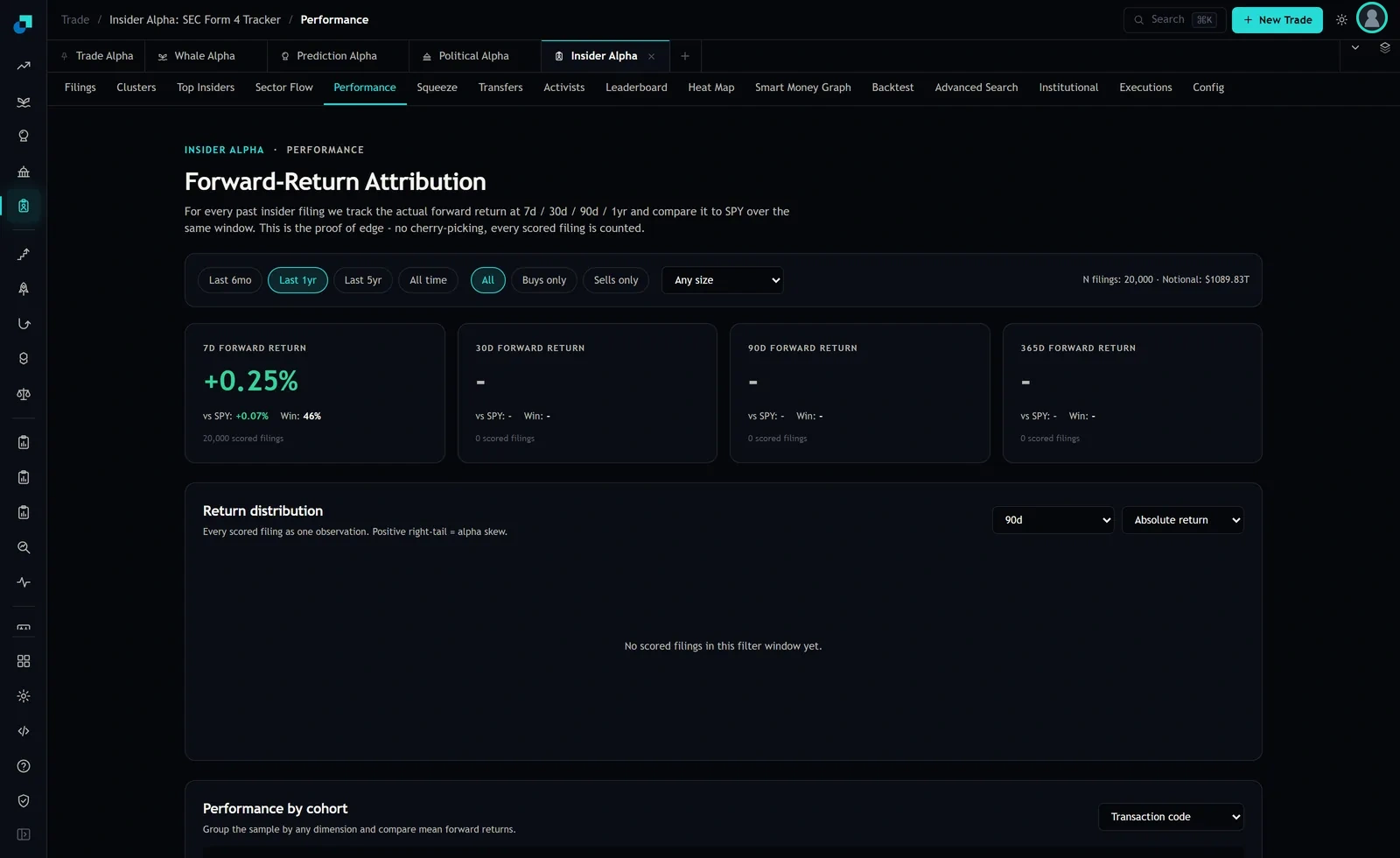
That gap is the whole reason for this article. The panel is answering whether the population of filings carries excess return over a week. A half-life estimate is asking how that excess is distributed across the minutes and hours after publication. The first cannot be refined into the second, and the size and side filters on the panel, which offer buys only, sells only, and thresholds at 25 thousand, 100 thousand, 500 thousand and one million dollars, define the population you would want to run the finer study on rather than substituting for it.
Building the intraday event clock
Five decisions define the estimator and each one moves the answer materially.
The event stamp. Use the acceptance datetime to the second. Record it in a single timezone with an explicit convention for daylight transitions, and keep the raw value alongside the normalised one so the conversion is auditable.
The first tradable moment. A large share of Form 4 filings are accepted after the close, so the first moment you could have acted is the next session's open, not the next second. Those two populations behave differently and must be estimated separately. Pooling them produces an average half-life that describes neither, and it systematically flatters the intraday estimate because the overnight cohort has its move compressed into the opening auction.
The benchmark. Subtract something at the same frequency you are measuring at. A daily benchmark applied to a minute-level event study leaves market drift inside the residual, and over a full session that drift is comparable in size to the effect being measured. A minute-matched index return or a sector proxy is the minimum.
The price series. Use quote midpoints rather than trade prices for the return calculation, or the bid-ask bounce will contaminate the first few observations exactly where the estimate is most sensitive. In illiquid names the spread is wide enough that this alone can generate an apparent instantaneous jump.
The window and the bins. Log-spaced bins from the first minute out to several sessions, since the interesting structure is at the short end and uniform bins waste resolution there.
Estimating the decay and reading the band
Fit excess return against elapsed time and report the half-life as the point where the modelled excess falls to half its initial value, with a confidence band rather than a point.
Two things will dominate the result. The first is the filter set. A half-life fitted across all filings is not the half-life of the filings you would trade, and if your process only acts on discretionary open-market purchases above a dollar threshold then that is the population to fit on. The panel's own size thresholds are a reasonable starting grid. Report the estimate separately per bucket and expect them to differ, because they are different events.
The second is skew. The 46 percent win rate on the panel, sitting alongside a positive mean, tells you the population return is carried by a right tail rather than by a majority of filings working. A decay curve fitted to means over that distribution is heavily influenced by a small number of observations, and the median decay and the mean decay can disagree about the answer. Fit both. If they disagree, the honest reporting is that the average filing decays one way and the filings that pay decay another, and the second is the one your sizing depends on.
What a slow book can still capture
The purpose of the estimate is a capacity decision, so express it in those terms rather than as a research finding.
Take the fraction of excess return still available at the point where your execution would realistically begin, given your participation-rate constraint and the liquidity of the names involved. Compare that residual, in basis points, against your all-in implementation cost for the same names. If the residual does not clear the cost with margin, the correct conclusion is that this signal is not tradable at your size, and that conclusion is worth reaching deliberately rather than discovering through a year of slippage.
Where the residual does clear, the sizing still has to respect the skew. A signal whose expected value comes from a right tail cannot be sized like a symmetric edge, because the same expected value carries a much higher chance of a long unprofitable stretch, and the review conversation during that stretch is far easier if the distribution was documented in advance. Write down the fitted half-life, the filter set it was fitted on, the date of the fit and the cost assumption, and refit on a schedule rather than after a bad quarter.