A signal engine sizes one trade at a time. A volatility target is a statement about a portfolio. Those two things live at different layers and the recurring mistake is to try to merge them, usually by pushing the volatility scalar down into the strategy's own parameters where it corrupts the thing it was supposed to be governing.
The correct arrangement is a seam, with the engine sizing its trades exactly as designed and an overlay adjusting quantity above it. Getting the seam in the right place is most of the work, and the reason it goes wrong is that the engine's sizing output and the overlay's sizing output are both denominated in the same units, so it is easy to apply one on top of the other without noticing what you have broken.
What the engine hands you and where the seam belongs
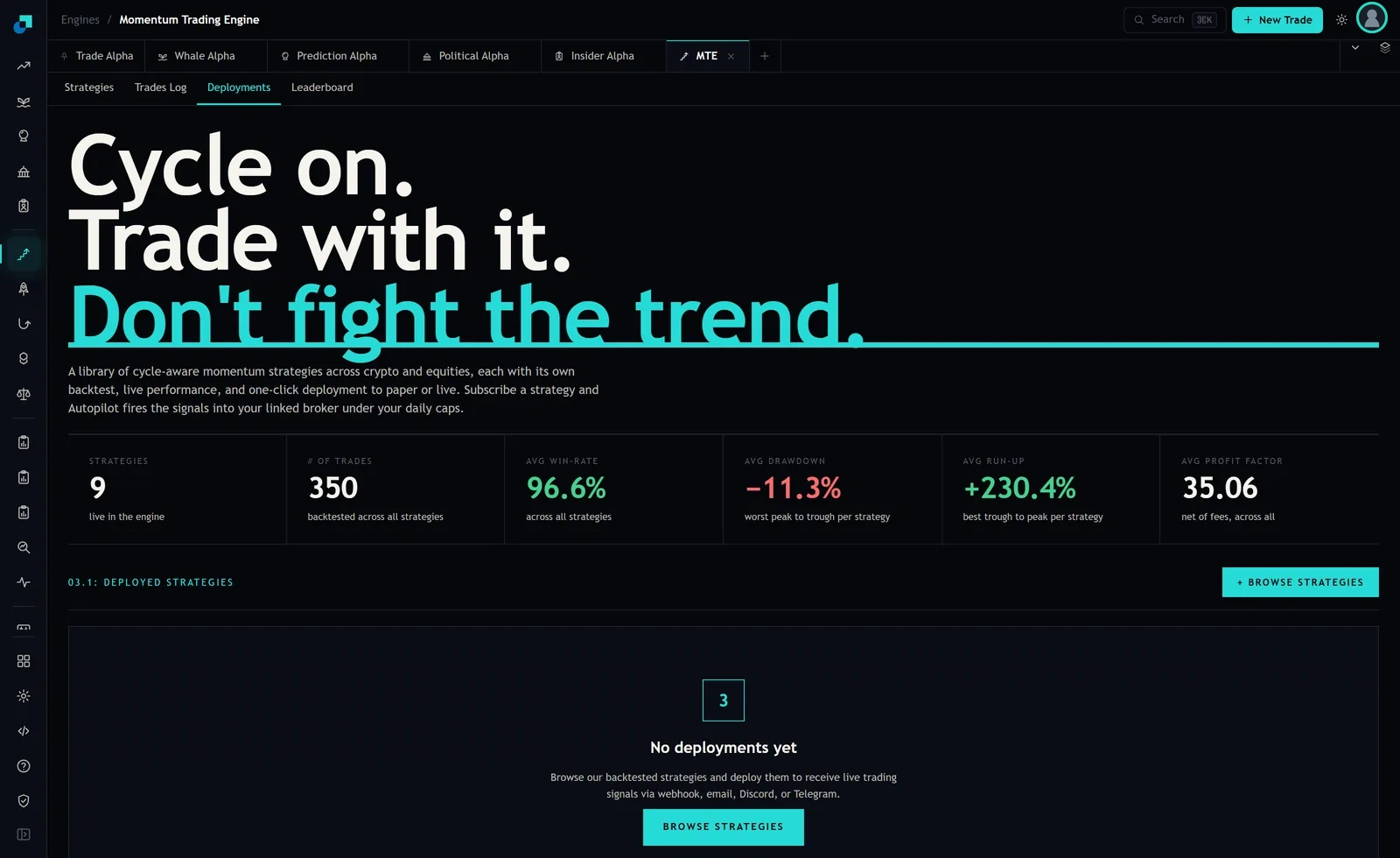
The Momentum Trading Engine's deployments tab describes the contract plainly. You browse the backtested strategies and deploy them to receive live trading signals via webhook, email, Discord or Telegram. The page description above adds that once a strategy is subscribed, Autopilot fires the signals into your linked broker under your daily caps.
Two guards, then, and both are per-account activity limits rather than risk measures. A daily cap constrains how much firing happens. Nothing in that pipeline observes the sleeve's realised volatility, and nothing could, because a per-deployment signal path has no view of the other deployments' positions.
So the overlay sits between the signal and the order. It receives an intended position from the engine and emits a smaller or larger quantity. That is the only place it can sit without either being blind to the portfolio or being invasive to the strategy. At capture the deployments panel was empty, reading "No deployments yet", which is the cheapest possible moment to specify this. Retrofitting an overlay onto a running sleeve means changing sizes on live positions, and that conversation is much worse than this one.
Scale the quantity, never the stop
Here is the rule, and it is the one thing to take away. The scalar multiplies quantity. It does not touch any price level the strategy computed.
Work it through. Suppose a strategy's own convention is to risk one percent of the sleeve per trade with a stop four percent away from entry. That implies a notional of twenty-five percent of the sleeve. Now the overlay measures the sleeve running at eighteen percent annualised volatility against a twelve percent target, so the scalar is twelve divided by eighteen, which is 0.667. Notional becomes 16.7 percent of the sleeve. Risk per trade becomes 0.67 percent. The stop stays four percent away from entry.
That last clause is the whole point. The trade's shape is unchanged: the same distance to the stop, the same distance to any target, the same probability of being stopped out. Only the size of the bet moved. Compare that to the alternative that people reach for, which is widening the stop to reduce the frequency of losses. Widening the stop changes the exit distribution, changes the win rate, changes the average loss, and means that the backtest the deployment was selected on no longer describes what is running. You have not applied a risk overlay; you have deployed a different strategy and called it risk management.
Three measurement choices that decide whether this works
The formula is trivial. The estimation is where the outcomes are actually determined, and there are three decisions to make explicitly rather than by default.
Which volatility. Realised volatility of the sleeve's own return series is the honest choice and it is backward looking. Ex-ante volatility from a position covariance matrix is forward looking and depends on a covariance estimate you may not be able to support. Per-strategy volatility summed without cross-terms is the wrong answer dressed as the right one. Pick one, write down why, and expect to defend the choice rather than the number.
Which window. A short estimation window produces a scalar that moves constantly, and every move is a trade with no signal content in it. Put a figure on that before choosing: on a fifty million dollar sleeve, a scalar that swings twenty percent between rebalances is ten million dollars of notional turnover generated purely by the estimator. On a low-turnover trend book that can exceed the turnover of the strategies themselves, at which point the overlay is the dominant cost centre.
Which trigger. Rebalance on a band, not continuously. Only re-scale when the scalar has moved more than a stated threshold from the level currently implemented, and state the threshold in the policy. Banding converts most of the estimator noise into no action at all, which is exactly what you want from a control layer.
Why the engine's own figures cannot feed the estimate
There is a tempting shortcut here that does not work, and it is worth closing off explicitly because the numbers are sitting right there on the page.
The engine's header tiles report an average drawdown of -11.3%, described as the worst peak to trough per strategy, and an average run-up of +230.4%, the best trough to peak per strategy, across nine strategies and 350 backtested trades in total. Those are per-strategy backtest extremes. A portfolio volatility cannot be derived from a set of per-component extremes under any assumption you would be willing to write down, because the cross-terms between components are the entire content of the calculation and are precisely what a per-strategy summary omits.
There is a second obstacle. A covariance estimate needs overlapping return series at a common frequency. What the engine publishes is trade-level records, and trades on different strategies start and end on different days with different holding periods. Converting a trade log into a daily return series per strategy is a piece of work you have to do yourself, from your own position and price files, and it is the actual prerequisite for any of this. Budget for it rather than assuming the data arrives in the right shape.
The failure modes to write into the policy in advance
Volatility targeting has two well-understood adverse behaviours and both should appear in the document before the first deployment, so that a bad quarter produces a conversation about whether the policy was followed rather than about whether it was ever a good idea.
The first is that it cuts into rising volatility even when returns are positive. There are regimes where volatility and return rise together, and the overlay will reduce exposure into them. That is not a malfunction, it is the mandate, and stating so in advance is what stops it being relitigated in the middle of it.
The second is arrival lag. Volatility clusters, so a realised estimate rises after the move that caused it. The overlay will therefore reduce size shortly after the loss rather than before it, and increase size shortly after the recovery. Over a sharp reversal it can do both at the worst moments. Banding and a longer window reduce the frequency of this without eliminating it.
Finally, cap the scalar's upside. A target with no ceiling levers a quiet market, and quiet markets are where gap risk accumulates unobserved. A maximum scalar of one, so the overlay can only ever reduce, is a defensible starting position for a first implementation and it removes the entire class of arguments about how much leverage the model was allowed to recommend.