The ladder story is one of the most durable pieces of folklore on a crypto desk. A token appears on a couple of second-tier venues, then a derivatives venue, then the majors, and everyone treats the early rungs as an early read on the late ones. Stated that way it is a story. Stated properly it is a conditional probability with a lag distribution attached, and the difference between those two framings is the difference between a feature and a narrative you are paying for.
What follows is the construction. I am not going to hand you a conversion rate, because the module does not publish one and I am not going to invent one. What I can do is specify exactly which number you should be computing, and name the four things that will make your first attempt at it wrong.
Turning the claim into something falsifiable
Write the hypothesis so that it can fail. The version worth testing is this. Conditional on a token receiving its first listing at a venue in tier B during month t, the probability of a first listing at a tier A venue within h days is materially higher than the corresponding probability for tokens matched on age, chain, market cap and liquidity that did not receive the tier B listing.
Three things are now nailed down that the folklore version left loose. There is a conditioning event with a date. There is a horizon. And there is a control group, which is the part almost everyone skips, because without it a high conversion rate might just be telling you that tokens which get listed anywhere are bigger and more liquid than tokens which do not.
You also need a tier definition, and it will not come from the data. There is no tier field in the feed. Write your tiers down as a static mapping with a rationale, freeze it before you run anything, and version it. A tier map edited after seeing results is not a feature, it is a fit.
What the feed supplies, and what it withholds
The listings module carries three streams, upcoming, listed and delisting. With all three enabled my capture showed 300 of 300 rows in the Exchange Listings Ledger, and the row schema was Symbol, Name, Pair, Exchange, Type, Chain, MCap, Volume, Liquidity, Conf%, Date, DEX and Trade.
Everything you need for the numerator of the sequence study is on that row. Symbol and chain for identity, Exchange for the venue, Type for the state, Date for the stamp. What is missing is everything else. There is no history, no per-token event timeline, and no field that links this listing to the same token's earlier listing elsewhere. The linkage is your join and it is not trivial, because the Symbol column is a ticker and tickers collide across chains and across unrelated projects.
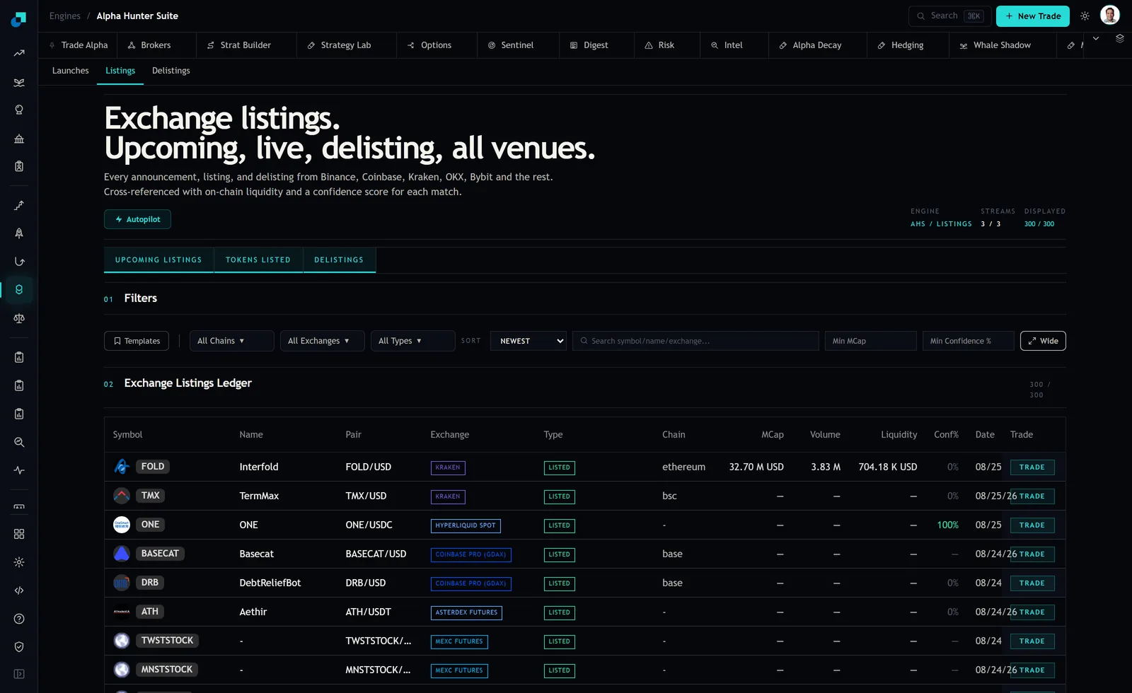
Resolve identity on chain plus contract address wherever the row gives you one, and treat rows where the chain shows a dash as unresolved until you have matched them by hand. In the capture, the two MEXC Futures rows and the Asterdex Futures row had a dash for chain and, in two cases, no Name at all. Those rows can still be events in your sequence table, but they cannot be joined automatically, and a study that silently drops them has already introduced a bias toward the venues with cleaner metadata.
Building the sequence table
One row per token, not per listing. The columns you want are the identity key, the first-observed date, the tier of the first listing, then a first-listing date per tier, then a terminal status field.
Three construction rules do most of the work.
- Membership in a cohort is fixed at the conditioning event and never revised. A token enters the tier B cohort on the day of its tier B listing, and it stays in that cohort whatever happens next, including going to zero.
- Every observation is right-censored at your data cut. A token that received its tier B listing twenty days ago has not had time to convert at a ninety day horizon, and counting it as a failure understates the rate while dropping it overstates it. Censoring is the correct treatment and it is what a survival estimator is for.
- Death is a competing risk, not a missing value. A token that loses all its liquidity has not failed to convert in the same sense as one that is alive and unlisted. Model them separately or your headline number blends two very different things.
The output you want is not a single percentage. It is a cumulative incidence curve, the share of the cohort that has received a tier A listing by day d, with the competing risk of token death handled explicitly, plotted alongside the same curve for the matched control cohort. The gap between the two curves is the feature. The level of either curve alone is not.
The four things that will make the first version wrong
Survivorship in the universe. If the feed does not retain rows for tokens that have died, a cohort you assemble retrospectively is a cohort of survivors, and survivors convert at a much higher rate than the population did. I would not assume the feed does or does not retain them. Check it directly by pulling rows from a date several months back and looking for entries with collapsed liquidity. If nothing dead is visible, your study starts on the day you begin taking your own daily snapshots, not on the day you decided to run it.
Reverse causation on size. Tokens do not receive top-tier listings because they were on a mid-tier venue. Both events are downstream of the token becoming large, liquid and legally clean. If you do not match on market cap and liquidity as of the conditioning date, you will measure size and call it sequence. Matching on the values as of the conditioning date, not current values, is the whole difficulty, and it is another argument for point-in-time capture.
Ticker collisions. A naive join on Symbol will merge unrelated tokens and manufacture sequences that never happened. This bias runs in your favour, which is what makes it dangerous.
Announcement versus effect. The Date field is a single date, and the distinction between when a listing was announced and when it became effective is not visible on the row. For a sequence study measured in days that difference is inside your resolution. Either widen the horizon until it does not matter or capture the underlying announcement times yourself.
What a real result would be worth, and where it stops
Suppose the curves separate and the gap survives the matching. You now have a conditional probability with a lag distribution, and the natural next step is a position rule. Two constraints bound how much that rule can earn.
The first is capacity, and it binds harder than the statistics do. A feature that fires on tokens whose on-chain liquidity is measured in hundreds of thousands of dollars cannot carry a position measured in millions, no matter how strong the conditional probability is. Compute the strategy's capacity from the depth of the names it selects, at your participation rate, over your intended holding period, before you compute anything else. Most sequence features die here rather than in the backtest.
The second is that this is a public observable. Anyone with the same feed can construct the same table. A feature built entirely on public event sequencing should be expected to decay as it is discovered, which means the honest way to run it is with a live measurement of the gap between the cohort curves, refreshed monthly, and a rule that retires the strategy when the gap closes rather than when the drawdown becomes uncomfortable.
Both of those numbers, the capacity and the current gap, belong in the strategy document alongside the original result. A desk that can produce them in a review is defending a process. A desk that can only produce the backtest is defending a story with error bars on it.