Liquidity overlays acquire a lead time the way codebases acquire magic numbers. Somebody runs a lag scan on a sample, one horizon fits best, that horizon goes into the specification, and within two years it is treated as a property of the world rather than as an artefact of a particular window. Then it stops working, the overlay is blamed, and the lag gets re-estimated on the newer sample and hard-coded again. The failure is not that the number was wrong. The failure is that the object was never a number.
What a hard-coded lead time actually asserts
Writing a fixed lag into a model asserts something quite strong: that the interval between a change in monetary conditions and its expression in asset prices is a constant of the system, invariant to the size of the impulse, the channel it travels through, the starting valuation of the assets receiving it, and the balance sheet capacity of the intermediaries in between. Stated that plainly, nobody would defend it. Stated as a parameter in a specification, it passes review routinely.
Two things go wrong in practice, and they compound.
The first is selection. A lag scan across a range of candidate horizons on a limited macro sample will always return a best-fitting horizon, because something has to win. With a handful of independent monetary episodes in the window, the difference in fit between the winner and its neighbours is usually well inside the noise. What gets recorded in the model documentation is the winner. What does not get recorded is that the runner-up was indistinguishable.
The second is that a point estimate propagates into the signal timing, the rebalancing calendar and the attribution window simultaneously. When the true lag drifts, the overlay does not degrade gracefully; it enters late, exits early, and the attribution window straddles the wrong period, so the performance report cannot even diagnose the problem. Three symptoms, one cause, and the review usually attributes them to three separate things.
The module itself declines to pick one horizon
There is a hint of the right posture built into the Regime tab. The Regime Heatmap panel is described as six liquidity factors scored across six time horizons, with darker shading indicating stronger readings, on a legend running from strong bullish through neutral to strong bearish.
Six horizons, not one. That construction implicitly concedes that a liquidity factor does not have a single relevant timescale, and it presents the factor-by-horizon grid rather than collapsing it into a single lead time. The header strip above it does the same thing in a different way, carrying a composite of 85 on a 0 to 100 scale alongside separate reads for LIQUIDITY on net flows, FUNDING on the SOFR and IORB relationship, and MARKETS on asset momentum, all printing NEUTRAL under a RISK-ON classification.
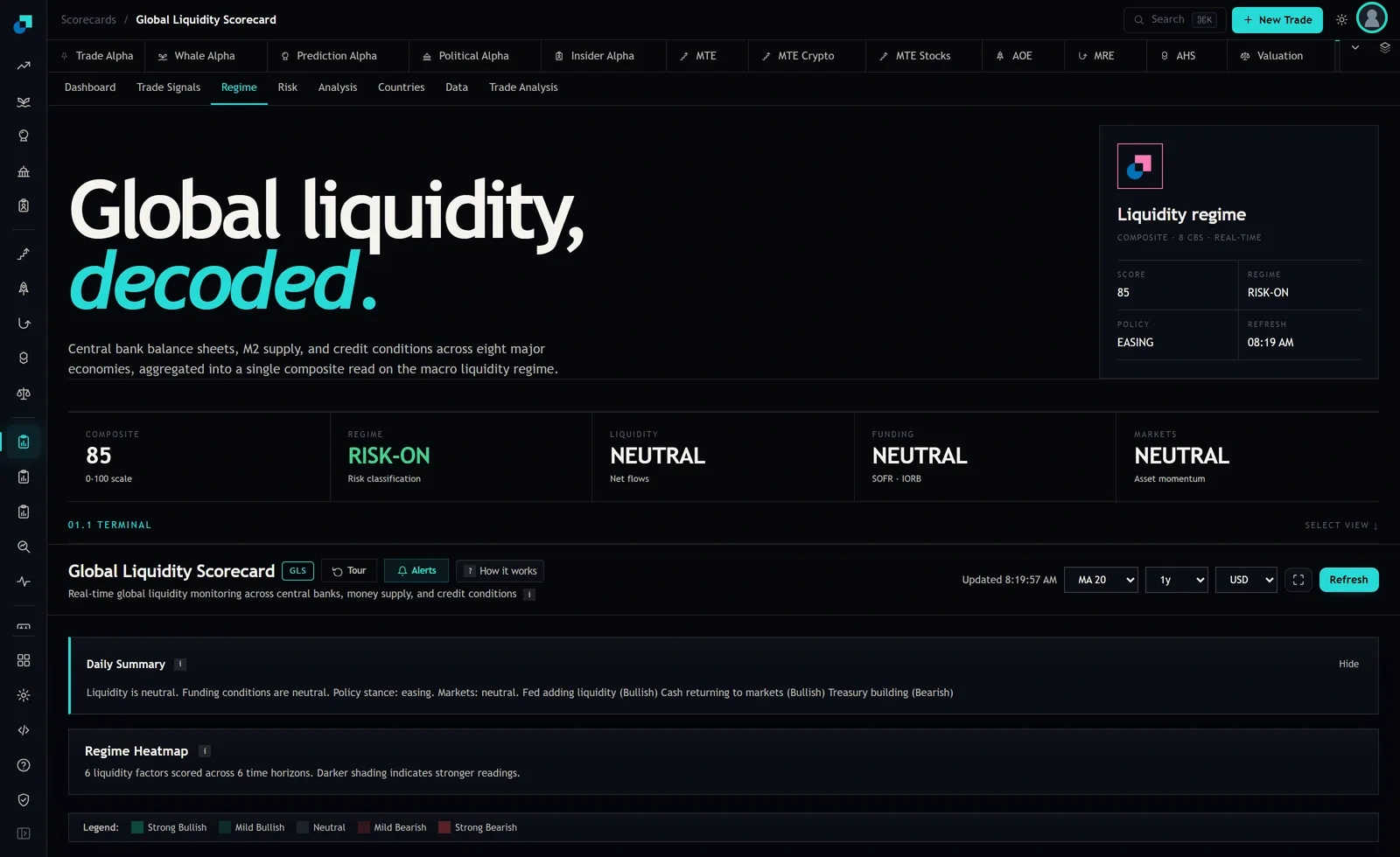
Those components have obviously different transmission speeds. A funding spread is a same-day object. An aggregate balance sheet is a weekly or monthly one. A composite that bundles both cannot have a single lag to anything, because its own constituents do not share a clock. That observation alone should be enough to retire the point estimate.
Estimating the lag as a distribution instead of a parameter
The practical replacement is a lag profile rather than a lag. Estimate the relationship at every horizon in a range and report the whole profile, with intervals, rather than reporting the argmax.
Four specification points decide whether the profile is informative.
- Work in first differences of the composite. It is bounded on a 0 to 100 scale and sits in ranges for long stretches, so a levels specification against a trending asset series produces a fit driven by shared drift rather than by transmission.
- Use non-overlapping windows where you can, and Newey-West errors with a lag matched to the overlap where you cannot. Overlapping horizon regressions on macro data generate t-statistics that are inflated by construction, and lag scans are unusually prone to this because the overlap grows with the horizon being tested.
- Correct for the multiplicity. Scanning twenty horizons and reporting the best one without adjustment is a guaranteed false positive generator. At minimum, report how many horizons were tested next to the result.
- Bootstrap the argmax. Resample the episodes, re-run the scan, and record which horizon wins each time. The spread of that distribution is the honest confidence statement about the lead time. If the winning horizon moves substantially across resamples, then the point estimate in your current model documentation is not a finding.
The output you want in the file is a chart of coefficient against horizon with its interval band, plus the bootstrap distribution of the argmax. In most macro samples that band will be wide enough that a broad range of horizons is statistically indistinguishable, which is the result, not a failure to find one.
One data caveat that invalidates this entire exercise if ignored. Balance sheet, monetary aggregate and credit series are revised. A lag profile estimated on restated inputs describes a sequence of readings nobody ever saw at the time, and lag estimation is far more sensitive to that than a levels regression is, because a revision shifts the timing of the very turn you are trying to locate. If you want a tradable claim, you need vintage data or an archive of the state as it printed.
What widens the distribution
Four conditions reliably stretch the profile, and knowing them lets you say something useful about the current environment rather than about the average one.
Impulse size. A small change in conditions has to work through preference and portfolio adjustments that take time. A large one forces balance sheet responses that are close to immediate. The same channel therefore transmits at different speeds depending on magnitude, which by itself makes the lag a function rather than a constant.
Intermediary capacity. Liquidity reaches assets through balance sheets that can be constrained. When dealer capacity is impaired, an expansion in aggregate conditions sits in reserves rather than reaching risk assets, and the lag lengthens or the transmission simply fails for a period.
Starting valuation. If risk assets already price the expected easing, the observed lag looks long or absent, because the transmission happened at the point of expectation rather than at the point of measurement. This is the single most common reason a lag estimated across one cycle fails in the next, and it is invisible in a specification that contains no valuation term.
Channel composition. A liquidity expansion driven by fiscal cash management transmits differently from one driven by asset purchases, and both differ from one driven by a compression in credit spreads. The Daily Summary panel on this tab names its drivers with directions attached, at capture including Treasury building marked bearish alongside two bullish drivers, which is exactly the compositional detail a single composite lag cannot represent.
Building an overlay that does not need a point estimate
The design implication is to stop asking the model for a date and start asking it for a state.
Trigger on persistence rather than on a lead. Require the composite to have moved and to have stayed moved for a defined number of readings before exposure changes. This is a specification whose behaviour is defined without reference to any lag, so it degrades gracefully when the transmission speed drifts.
Scale the exposure change to the confidence in the profile rather than to the point estimate. Where the bootstrap distribution of the argmax is tight, the overlay can carry a larger share of the risk budget. Where it is diffuse, the same signal should move less. That linkage puts the model risk into the sizing, which is where a committee can see it.
Report the profile in the review, not a single lag. The sentence you want on the record before a bad quarter is that the transmission interval is estimated as a range, that the range is wide on the available sample, and that the overlay is sized accordingly. That sentence is defensible after the fact. A model document containing one number and no interval is not, and the meeting where you discover this is not the meeting to find out.
Finally, re-estimate the profile on a schedule and record each vintage. If the profile is stable across successive estimations, that stability is a genuine finding and worth acting on. If it wanders, you have learned that the parameter your predecessors hard-coded was never there to begin with, which is worth more than a better guess at its value.